Anomaly Detection with Z-Score: Pick The Low Hanging Fruits

This article introduces an unsupervised anomaly detection method which based on z-score computation to find the anomalies in a credit card transaction dataset using Python step-by-step.

Anomaly detection techniques can be applied to resolve various challenging business problems. For example, detecting the frauds in insurance claims, travel expenses, purchases/deposits, cyber intrusions, bots that generate fake reviews, energy consumptions, and so on.

Unsupervised learning is the key to the imperfect world because in which the majority of data is unlabeled. It is also much harder to evaluate an unsupervised learning solution than supervised learning method which we will discuss in details later on.

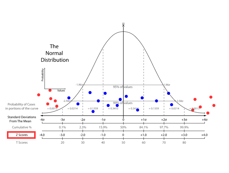
The hypothesis of z-score method in anomaly detection is that the data value is in a Gaussian distribution with some skewness and kurtosis, and anomalies are the data points far away from the mean of the population.

To make it intuitive, the following image was adapted from Standard score wiki page. The blue dots represent inliers, while the red dots are the outliers. The larger the number of standard deviations from the mean, the more anomaly the data point is. In other words, the further away from centre, the higher probability to be an outlier.

The core idea is so straightforward that applying z-score method is like picking the low hanging fruits comparing to other approaches, for example, LOC, isolation forest, and ICA. It is also practical to use z-score as benchmark in the unsupervised learning system which should ensemble multiple algorithms for the final anomaly scores.

Quick glance at the dataset

The credit card fraud detection dataset can be downloaded from this Kaggle link.

The shape of the dataset is (284807, 31).

“Time”: Number of seconds elapsed between this transaction and the first transaction in the dataset

“Amount”: Transaction amount

“Class”: 1 for fraud, 0 otherwise

“V1” ~ “V28”: Output of a PCA dimensionality reduction on original raw data to protect user identities and sensitive features

Check the completeness. There is no missing value which saves some work for us.

Compute the skewness of the dataset. As shown below, there are 1.72 fraudulent transactions in every 1000 entities.

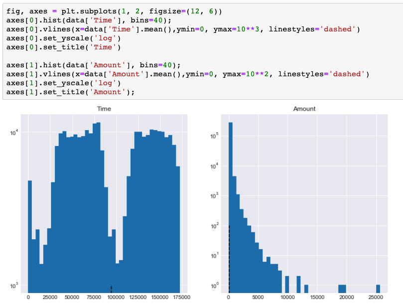
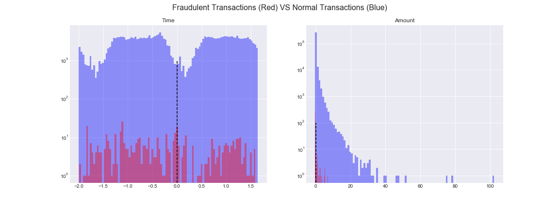
Visualize the distribution of variables “Time” and “Amount”.

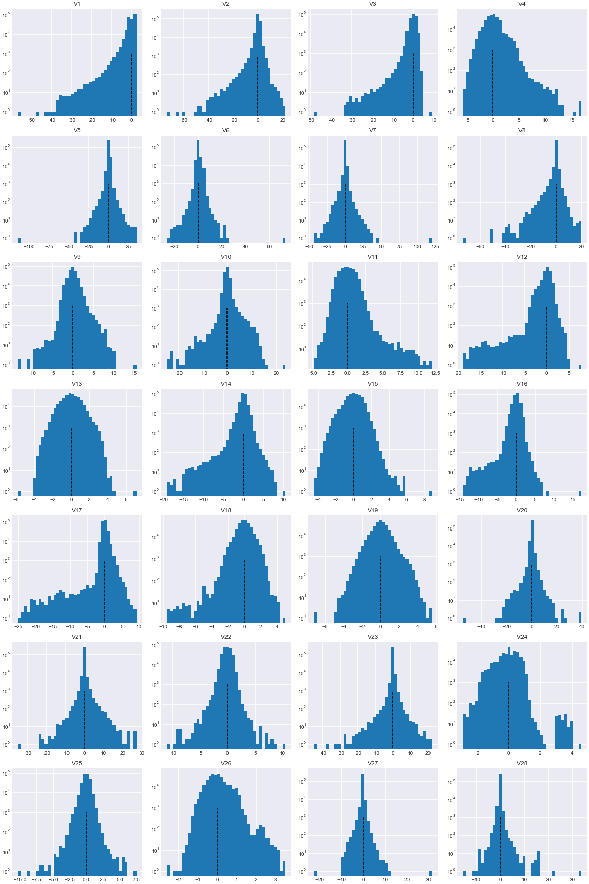
Visualize the distribution of variables “V1” to “V28”.

Feature scaling with standardization

As illustrated in the figures above, real life data rarely follows a perfect normal distribution. More than that, features “Time”, “Amount”, and “V*”s are sitting at different scales.

The code below will standardize the features except “Class” so that these features would be centred around 0 with a standard deviation of 1. I would like to emphasize that standardizing is an important step and also a general requirement for many machine learning algorithms.

Feature selection by visualizing outliers/inliers distribution

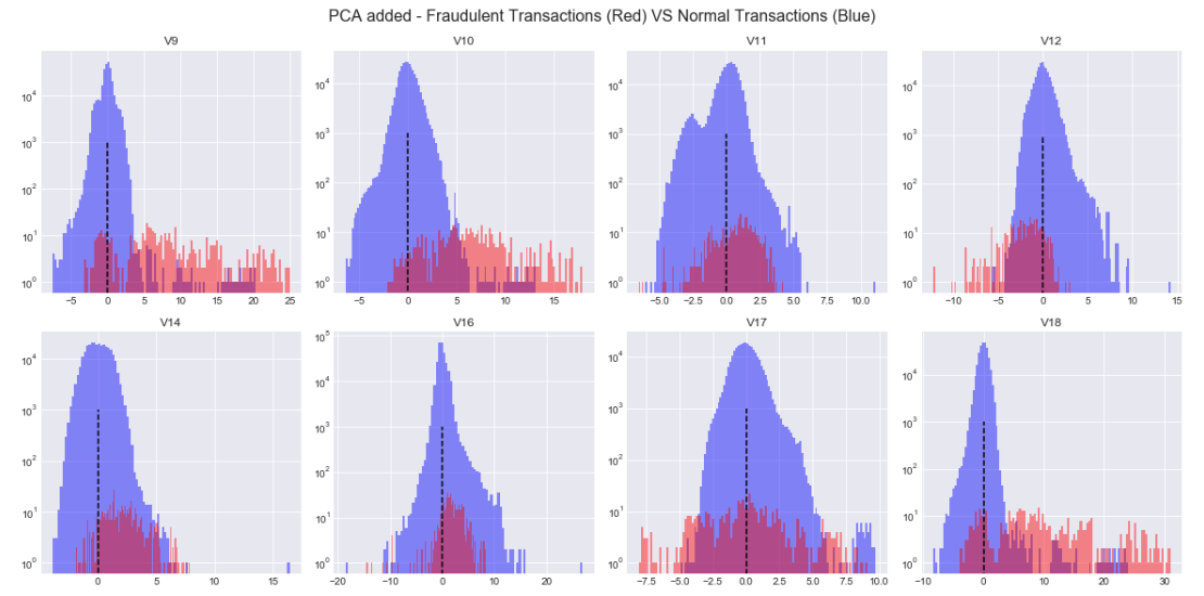
The red bars represent the fraudulent transactions while the blue bars are the normal transactions.

We can see that some features are not able to separate the outliers from inliers, for example, “Time”, “Amount”, “V19”, and “V26”. The red (outliers) are overlapped with blue bars (inliers). These features could not be feed into z-score models due to they could not differentiate the red from the blue.

Base on the same theory, I would pick features [“V9”, “V10”, “V11”, “V12”, “V14”, “V16”, “V17”, “V18”] and ignore the others. We can expect it to be able to pickup a good portion of anomalies which relies on the “intersections” among these cases.

PCA transformation and feature selection II

Perform the PCA transforming to get a dimensionality-reduced dataset even though I set the n_components to 8 that we did not reduce the dimensionality.

From the plot below, we can see that features [“V11”,”V14″,”V16″] could not separate the blue and the red obviously that they will be excluded before feeding the model.

Build and train the z-score model

1. Build and run a z-score model to get the anomaly score for each feature.
2. Then averaging the score of each feature into an overall score for all features which is stored in column “all_cols_zscore”.
3. After that, concat the score dataset with the label “Class”: 1 for fraud, 0 otherwise.
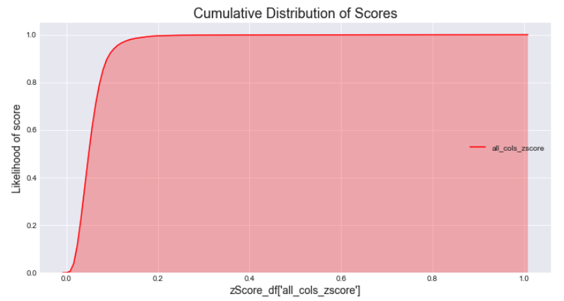
4. Check the Cumulative Distribution of the scores we computed.

# plot the cumulative histogram
fig2, ax2 = plt.subplots(figsize=(12, 6))    
x = zScore_df['all_cols_zscore']
ax2 = sns.kdeplot(x, shade=True, color="r", cumulative=True)# tidy up the figure
ax2.grid(True)
ax2.legend(loc='right')
ax2.set_title('Cumulative Distribution of Scores', fontsize = 18)
ax2.set_xlabel('zScore_df[\'all_cols_zscore\']', fontsize = 14)
ax2.set_ylabel('Likelihood of score', fontsize = 14);

As illustrated in the cumulative distribution of scores, around 90% of the scores are smaller than 0.1; almost 100% of the scores have value under 0.2.

Label your prediction

Fun part! How to label the prediction with the scores we got above?

1. Sort the dataset by “all_cols_zscore” descendingly because the higher the score, the more abnormal.
2. Label the top 350 rows with ‘predictClass’ label equal to 1, while the rest with 0 which means we predict the top 350 entities as fraudulent transactions.
3. Calculate and printout the precision and recall.

• The shape of the training dataset is 190820 rows with 5 features.
• There are 1.72 fraudulent transactions in every 1000 transactions.
• The precision when we label 350 cases as frauds is 55.14% which means that if we predict 100 transactions as frauds, 55.14 cases out of them are fraud in reality.
• The recall when we label 350 cases as fraud is 58.48% which means that if there are 100 fraudulent transactions, 58.48 cases can be successfully detected by the algorithm.

The result seems a bit poor. To be honest, it is a highly skewed dataset that we are looking for a needle in a haystack. The performance is not ideal but good enough in the real business world.

One step further: evaluate with multiple thresholds

We evaluated the model when label the top 350 entities with highest score as frauds. What if we label top 400, 450, 500,… cases as frauds? How will the z-score method perform under different thresholds?

1. Create the threshold list used for labeling.
2. Calculate and printout the precision and recall under multiple thresholds.
3. Save the precision and recall in the performance dataset.

By comparing the precision and recall under different thresholds, you could pick an appropriate threshold for your project. Precision means the purity of your prediction, and recall represents the completeness in detection.

In practice, I would suggest to lean a bit more on recall than precision because anomalies are usually rare in the population and you would like to catch as many anomalies as possible.

Run on the test dataset

How would our z-score method perform on never seen data? Let’s run it on the test dataset.

Impressively, it performs better on the test dataset with 67.90% recall when set threshold to 0.17%. For every 100 fraudulent transactions, we are able to catch 67.90 frauds out of them using the z-score method we built.

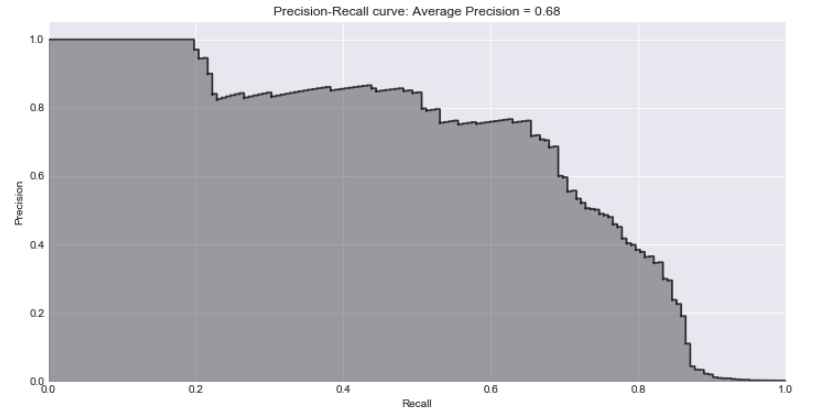
Compute average precision (AP) from prediction scores stored in “all_cols_zscore”.

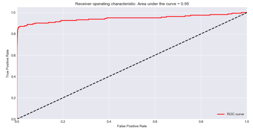
Plot ROC curve.

Conclusion

Yeah! We go through a lot of interesting things in this article. To recap, we talk about:

• the core idea of z-score method in anomaly detection
• feature scaling with standardization
• feature selection and PCA transformation
• build and train the model on train/test datasets
• evaluation with multiple thresholds

Actually, not that many after we summarized them. Anyway, the procedure used above is:

standardization -> feature selection I -> PCA -> feature selection II -> train model -> evaluation -> run on test data -> evaluation

You could run experiments using other possible procedures, for example,

• procedure I: standardization -> train model
• procedure II: standardization -> PCA -> train model
• procedure III: standardization -> feature selection I -> train model

The goal is that by comparing the precision and recall of each procedure, you can build a sense that how standardization, feature selections and PCA can significantly affect the performance of same model.

Unfortunately, for unsupervised learning problem in real world, because the absence of labels, we could not select features by visualizing the distribution of outliers VS inliers against each features. Usually the underlying business process should give us a sense of which features should be more relevant when we don’t have labels. Be mindful of the potential bias and variance though.

To summarize, if there is only one thing you would take away, it should be: the procedure for anomaly detection in supervised learning using z-score method

standardization -> feature selection I -> PCA -> feature selection II -> train model -> evaluation -> run on test data -> evaluation

the procedure for anomaly detection in unsupervised learning using z-score method

standardization -> train model -> evaluation -> run on test data -> evaluation