PCA reduces the dimensionality of data points that are in many spaces. Some ready codes and libraries allow coders to create PCA easily, however, do you know what is PCA and how does it work mathematically?

“The main idea of principal component analysis (PCA) is to reduce the dimensionality of a data set consisting of many variables correlated with each other, either heavily or lightly, while retaining the variation present in the dataset, up to the maximum extent.”

Intuitively, Principal Component Analysis allows us to see the position of data points with a lower-dimensional picture. It can be called a projection or “shadow” of these data points when the user looks from its most informative viewpoint, as a shadow of the diamond picture above.

If someone asks you what is PCA, these are the first things that you should keep in your mind about PCA.

• reduces dimensions
• tries to keep the maximum variance in dataset
• sometimes, new dimensions are not explainable.
• improving visualization

How does PCA work mathematically?

On the internet, the mathematical part of PCA is rarely explained step by step. There are very few resources about it and most of it not even detailed enough. I believe mathematical intuition allows us the connect puzzle pieces in the long term. Therefore now below you can see step by step calculation of PCA with an example.
Let’s say we have a dataset about exam scores of 5 students for their different sport lessons and we will try to reduce the dimension of this dataset.

1- Take features of the dataset, don’t consider Label.

PCA works on feature dimensions which are sport lessons in this case. Therefore, we shouldn’t consider a label column and unique student id’s. This process is only related to features of the dataset. After implementing all steps, the new scores of each student in PCA selected dimensions will be an outcome.

2- Normalisation of Your Dataset

PCA is a practice to change the direction of components to maximum variance directions. Basically, the original data will be allocated in different directions that maximize the variance. If you don’t normalize your dataset, the PCA technique can be biased toward specific features.

Normalization is done in two steps:

• First of all, subtracting the respective means of the variable from every data point. This produces a dataset whose mean is zero.
• Secondly, after subtracting means, dividing every data point to standard deviation. (which I will not implement in this article)

You can see the mean of every column as below:

3- Calculate Covariance Matrix

Before we get started, we shall take a quick look at the difference between covariance and variance. Variance measures the variation of a single random variable (like the height of a person in a population), whereas covariance is a measure of how much two random variables vary together (like the height of a person and the weight of a person in a population).

The normalization of data points is linked with the covariance matrix. Because in the covariance formula, the mean of every column (feature) needs to be subtracted from each data point of each attribute. If you apply normalization, the mean will be zero. If you don’t apply the first step of the normalization, it will be done by the covariance matrix formula.

Covariance calculation should be happening in every combination of two features.

If we say, we have d dimension ( d number of features), the covariance matrix will be in dxd dimensions.

• It is a square matrix
• It is a symmetric matrix from diagonal, therefore cov(X,Y) = cov(Y,X)

cov(X, X) indicates the variance of X feature. The bigger number indicates higher variance. Therefore the diagonal part of the matrix indicates the variance of each feature. Every other element in the matrix indicates the covariance of two different variables.

In our example, you can see the A matrix and mean of every column.

Therefore, the implementation for one of the values for the covariance matrix:

Cov(X,Y) = [(6–5)*(4–5.6) + (8–5)*(3–5.6) + (5–5)*(8–5.6) + (4–5)*(5–5.6) + (2–5)*(8–5.6) ] / (5–1)

What does this covariance matrix tell us?

• Higher variability is in running (+7.7 ) and lowest variability in tennis (+5.0) lectures.
• The covariance between volleyball and running is positive (as 0.35), this means the scores tend to covary in a positive way. As scores in tennis go up, scores in running tend to go up too, and vice versa.
• Covariance between tennis and volleyball is negative (as -4), this means the scores tend to covary in a negative way. As scores in tennis go up, scores in volleyball tend to go down, and vice versa.
• If the covariance of any two features were zero, it means that no predictable relationship between the movement of related two lessons’ scores.

4- Calculate EigenValues

Eigenvalue is a scalar that is used to transform (stretch) an Eigenvector.

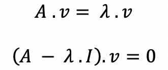
A is a square matrix (which is covariance matrix A), v is an eigenvector, λ is a scaler which is eigenvalue (associated with eigenvector of A matrix.
When you carry the right side of the question to the left side, you need to solve the below equation to get λ eigenvalue.

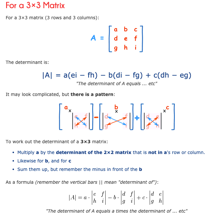
Now, we need to get λ values by solving the above equation. How to solve determinant of 3X3 dimension is in below Picture, but for more information please read this link.

Therefore, at the end our equation is equal to almost the below equation:

After solving this equation, you will reach to:

5- Calculate Eigenvectors

Intuitively, an eigenvector is a vector whose direction remains unchanged when a linear transformation is applied to it.

After finding Eigenvalues, now is the time for finding eigenvectors. You may remember our equation in the beginning was:

Now, we know A and λ. Now the question is which vector after dot multiplication with (A — λ) matrix gives zero?
For every λ value, we will find different eigenvectors. Let’s start:

(A- λ.I) = B , where B matrix is equal to A minus eigenvalue matrix.

By solving this equation, we will find Eigenvectors corresponding to eigenvalues. Eigenvalues = [λ = 11.0 , λ = 6.4 , λ = 0.58 ], and corresponding eigenvectors will be:

6- Sort and Select

Sort the eigenvectors by corresponding to decreasing eigenvalues and choose first n eigenvectors with the largest eigenvalues.

Eigenvectors only define the direction of new dimensions in the space. Therefore eigenvectors are unit vectors. We need to form our dataset according to these vectors.

Our goal by using PCA was the creation of fewer dimensions, therefore we will select a number of eigenvectors according to the number of dimensions that we desired.

Sort the eigenvalues corresponding to eigenvalues from highest to lowest. For example, if you want to decrease the dimension to two from three, then take the first two eigenvectors which are corresponding to the first two highest eigenvalues.

6. Create final data points with an eigenvectors matrix.

The end goal of Transform the real dataset onto the new subspace, with this we can have all students’ information into 2 dimensions. We need to dot multiply normalised dataset and eigenvector matrix created by taking highest eigenvalues. In matrix multiplication, the number of columns in the first matrix should be equal to the number of rows of a second matrix.

(3 columns x 5 rows) matrix will be dot multiplied by (2 columns, 3 rows) matrix to get transformed dataset in new dimensions.

(Normalised A matrix) . (Eigenvector Matrix) = Transformed Dataset

• Red squares indicates which row is multiplied by which column to get first element in new dimensions according to eigenvectors.

To conclude, you can see the latest dataset per student in 2 dimensions as determined by PCA and the same labels from the original table.

Please leave me a comment if you have any feedback !

Note: The real numbers are indicated until 2 digits after dot.